Overview
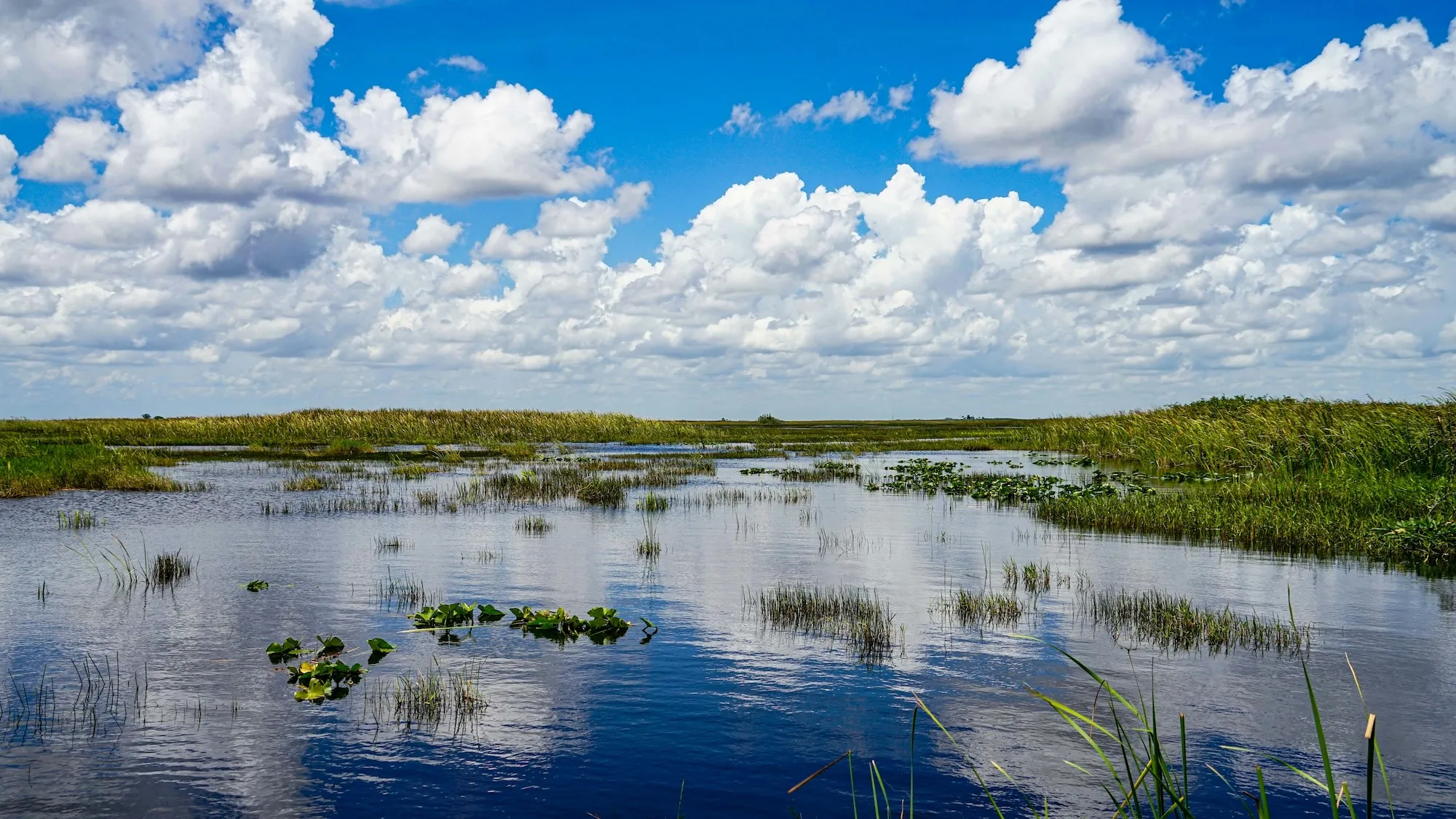
When a ship moves through shallow water, part of the powerful water jet generated by its propeller is pushed downward toward the bed. In a canal where dense salty water sits at the bottom under lighter fresh water, this jet can break up that layering and mix the two together. This blog shows exactly that process using a 3D hydrodynamic model of a 10 m deep navigation canal with a 100 ppt hypersaline layer sitting at the bottom ~1 m (Table 1). Two ships travel in opposite directions through the channel, and the model tracks how their propwash jets stir and mix the water column over one hour. Figure 1 shows the horizontal model grid along with the ship vessels’ initial locations and tracks.

Table 1 - Model properties
| Property | Value |
|---|---|
| Horizontal grid | 6,000 active cells |
| Vertical layers | 30 sigma layers |
| Active modules | Hydrodynamics, Salinity, Sediment Transport, Propwash |
| Simulation period | 1 hour |
| Ships | C-Tractor 13, C-Tractor 14 |
| Initial bottom salinity | 100 ppt in the 3 lowest sigma layers (≈1 m) |
2DV Animations: Velocity Vectors & Salinity
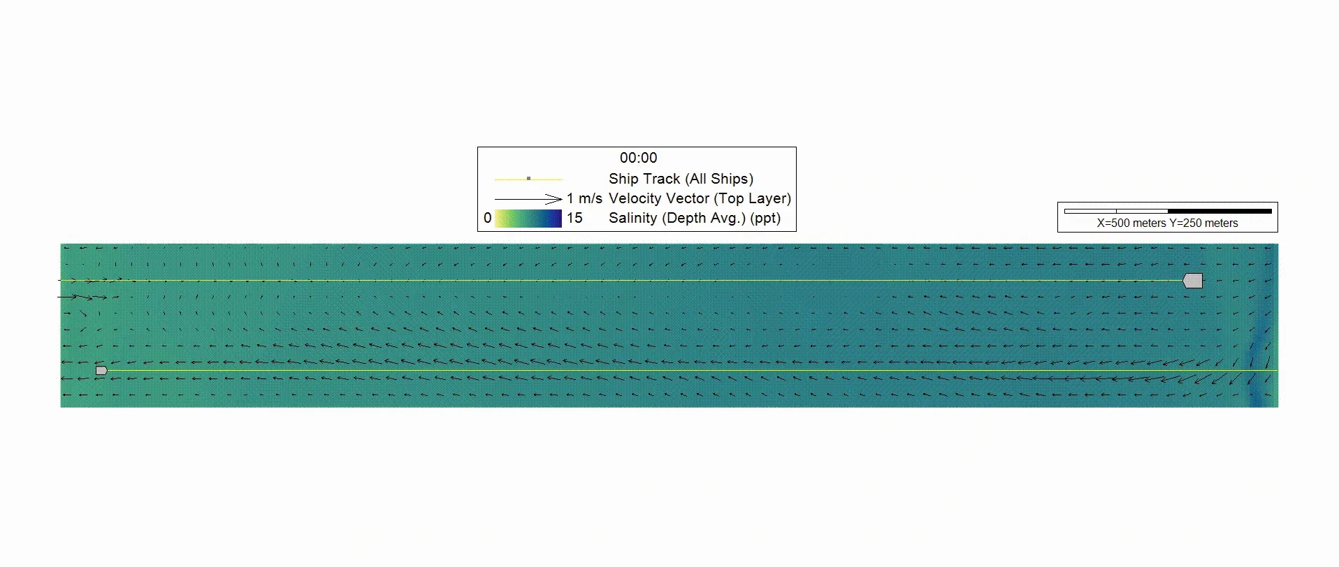
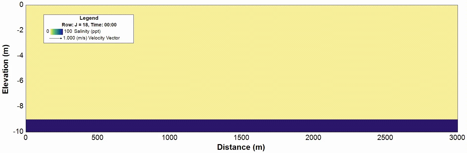
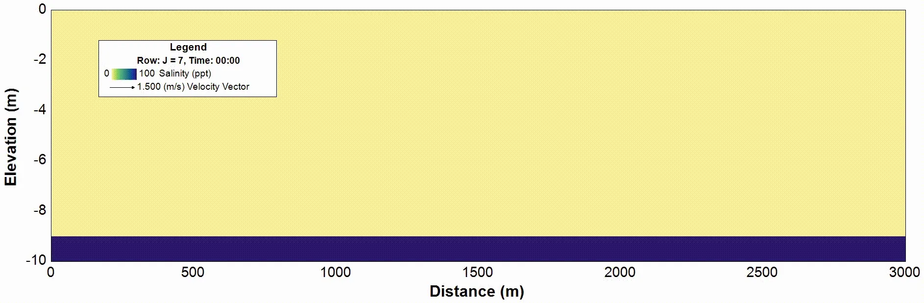
The three animations below show the model results from different viewpoints. In all of them, color represents salinity with yellow showing fresh water (0 ppt) and dark blue showing the dense hypersaline water (100 ppt). The arrows show water velocity.
Animation 1 shows the 2DH view of the depth-averaged salinity and the surface velocity vectors. As each ship moves through the channel, the propwash stirring the water on either side of the vessel track is visible. The salinity signature (patches of mixed water spreading laterally) shows where the hypersaline bottom layer has been lifted and blended into the water column above.
Animations 2 and 3 show the 2DV view along the path of C-Tractor 14 and 13 respectively. The downward propeller jet is visible as a concentrated cluster of eastward-pointing arrows for C-Tractor 14 and westward-pointing arrows for C-Tractor 13 that intensifies as the ship passes through the frame. When the jet hits the bottom, it fans out sideways and pushes the dense saline layer upward. After the ship passes, you can see the sharp boundary between the salty bottom water and the fresh water above has been replaced by a blended transition zone few meters thick.
Conclusion
The simulation shows that propeller action can be a major contributor to vertical mixing in stratified navigation canals. Even a single transit is enough to break up a sharp salinity boundary that would otherwise persist for hours. The 100 ppt hypersaline layer, initially confined to the bottom meter of the water column, is partially lifted and blended into several meters of depth by the time each ship has passed.
Using 30 sigma layers gives the model enough vertical resolution to track the gradual erosion of the halocline in detail which would be lost with a coarser setup. This kind of simulation can support decisions about navigation channel design, dredging assessment, and the management of water quality in port environments where stratification plays an important role.
Talk To The Experts