EFDC+ Explorer
A Pre- & Post-Processor for the Environmental Fluid Dynamics Code
Temporal Analysis
EE’s temporal analysis tools enable you to visualize model variables and compare them against observed datasets over time. Through time series plots, animations, and residual fields, you can track how concentrations evolve and assess alignment with calibration targets.
Time Series
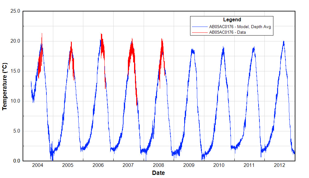
Time series plot for observed temperature data (red) and model output (blue) for the Little Bow River.
Time Series
Time series plots provide a clear, side-by-side comparison of simulated and observed data, making it straightforward to identify trends, discrepancies, and long-term patterns in model performance.
Animations
Animation of thermal plume releases from a power station's once-through cooling system.
Animations
EE’s 3D visualization engine supports rich, dynamic animations — including planar slices through the X, Y, or Z axes, parameter-based blanking, flight path rendering, and more. For example, the animation shown here illustrates EFDC+-simulated thermal plumes generated by a nuclear power station’s once-through cooling system, capturing the spatial extent and behavior of heat dispersion over time.
Time-Averaged Results / Residual Fields
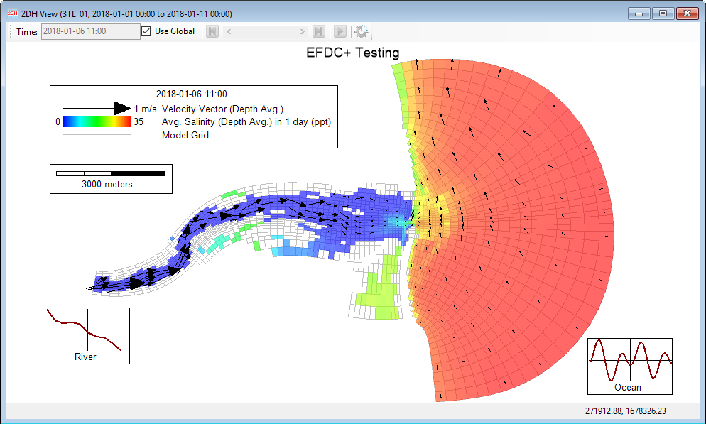
Time-averaged salinity using the mean mass transport feature in EE.
Time-Averaged Results / Residual Fields
Residual flow fields — user-defined, time-block-averaged outputs — allow you to cut through short-term variability and focus on the underlying, longer-term dynamics of a waterbody. By filtering out transient signals such as tidal forcing or other high-frequency boundary conditions, these fields reveal the dominant processes that would otherwise be obscured. Residual fields can also be animated for further insight.
The estuary example shown here displays a 24-hour averaged salinity field with flow direction overlaid, demonstrating how this feature simplifies the interpretation of tidal systems and helps isolate persistent circulation patterns.