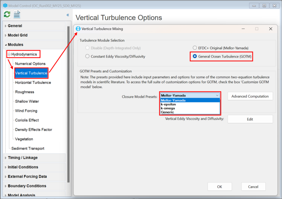
Starting from EEMS version 12, users have the flexibility to construct models using turbulence closures sourced from GOTM (General Ocean Turbulence Model) for vertical turbulence, in addition to the original EFDC+ options. This enhancement grants users more options and control when building their models within EEMS.

GOTM is a one-dimensional water column model for the most important hydrodynamic and thermodynamic processes related to vertical mixing in natural waters. In addition, it has been designed such that it can easily be coupled to 3-D circulation models and used as a module for the computation of vertical turbulent mixing (Umlauf et al., n.d.). It is a core component of other popular coastal and ocean models such as FVCOM, TELEMAC, and GETM.

The core of the model computes solutions for the one-dimensional versions of the transport equations of momentum, salt and heat. The key advantage of GOTM lies in its extensive collection of thoroughly tested turbulence models that have been integrated into the code. These models cover a wide spectrum, ranging from simple predefined expressions for turbulent diffusivities to intricate Reynolds-stress models involving multiple differential transport equations for resolution. While it may not be feasible to include every turbulence model published in oceanography, GOTM ensures representation from each relevant model family, encompassing empirical models, energy models, two-equation models, Algebraic Stress Models, K-profile parameterizations, among others (Umlauf et al., n.d.).

For more details on GOTM, the readers are recommended to consult the GOTM website for the source code, documentation, and test scenarios.

Turbulent closure methods play a vital role in the field of fluid dynamics, particularly in addressing the complex nature of turbulent flows. Turbulence, characterized by chaotic and unpredictable motion, occurs widely in various natural and engineered systems. However, directly simulating all the turbulent scales computationally is often impractical due to their vast range and high computational costs. Turbulent closure methods aim to model the effects of these unresolved turbulent scales by introducing simplified equations, which can be readily solved along with the governing equations. These methods are grounded in statistical theories and utilize empirical data to estimate the turbulence characteristics. Despite their inherent assumptions and limitations, turbulent closure methods have significantly advanced our understanding of turbulence and continue to be refined to improve the accuracy and efficiency of turbulent flow simulations.

There are different possibilities in the GOTM to compute scales q (or k) and l, which are related to turbulent kinetic energy and length-scale in turbulence. Respectively, turbulent kinetic energy refers to the energy associated with the random motion of fluid particles in a turbulent flow and is defined as the average of the squared velocity fluctuations in three spatial directions and length-scale represents the size of turbulent eddies or structures present in the flow and is important in determining the energy transfer and dissipation rates associated with turbulence, The models implemented in GOTM to compute these two parameters are categorized based on their complexity:

• Algebraic models: In this level, both k and l are computed using algebraic relations based on simplified forms of the transport equations. The length-scale may be prescribed empirically, making these models overly simplified for many situations.
• One-equation turbulence models: The one-equation models calculate the turbulent kinetic energy k with a transport equation whereas the turbulent length scale l is calculated with an algebraic expression. These models are popular in geophysical modeling.
• Two-equation models: The two-equation models compute both k and l from differential transport equations. The length-scale is usually determined indirectly through related variables like the rate of dissipation or the product kl. The primary advantage of two-equation models lies in their generality, as they can handle various fundamental flows that cannot be accurately simulated with algebraical length scales. Examples include the temporal decay of homogeneous turbulence, turbulence behavior in stratified homogeneous shear flows, and the spatial decay of shear-free turbulence from a planar source (Umlauf et al., n.d.).

Additionally, GOTM supports an ordering scheme for the extent to which transport equations for turbulent fluxes are solved and the assumptions made for stability function, which depending on the level of turbulent closure, these stability functions can be either constants, empirical functions, or functions of some non-dimensional flow parameters resulting from a higher-order turbulence model:

1. Standard models assume constant values for stability functions, leading to isotropic relations that may not be suitable for anisotropic flows.
2. Empirical functions of non-dimensional flow parameters are introduced for stability functions, attempting to reduce issues with the standard models.
3. More consistent models involve solving simplified forms of transport equations for Reynolds-stresses and turbulent heat fluxes in addition to k and the length-scale variable. This approach leads to the existence of vertical eddy diffusivities as a consequence of the model (Umlauf et al., n.d.).

Turbulence models in GOTM that are implemented in the EFDC include the adaptation of a generic length scale (GLS) approach to two-equation turbulence models suggested by Umlauf & Burchard, (2003). The first equation in the GLS model is the standard equation for transport of turbulent kinetic energy, and the second equation is for a generic parameter that is used to establish the turbulence length scale. These scenarios aim to constrain model parameters and derive a closed set of coefficients.

• Generic Model: Umlauf & Burchard, (2003) proposed a set of standard physical situations to evaluate standard two-equation models. To address this, they grouped two-equation models and recommended a coefficient set for a generic model.
• Mellor-Yamada 2.5 Model: The Mellor-Yamada 2.5 model is a two-equation turbulence closure method proposed by Mellor & Yamada, (1974) that considers both the turbulent kinetic energy and the turbulent kinetic energy dissipation rate. It is often used in atmospheric and environmental modeling, providing reliable predictions in a wide range of flow conditions.
• k-ε Model: The k-ε model is a two-equation model proposed by Rodi, (1984) that predicts the turbulent kinetic energy (k) and its dissipation rate (ε), making it suitable for a wide range of engineering applications.
• k-ω Model: The k-ω model is a two-equation model proposed by Wilcox, (1988) that employs the turbulent kinetic energy (k) and the rate of dissipation of energy per unit volume and time (ω) as the primary turbulence variables, offering improved performance in boundary layers and near-wall regions compared to the k-ε model.

Each of these methods has its strengths and weaknesses, and their suitability depends on the specific characteristics of the turbulent flow being simulated and the available computational resources.

Comparing turbulence models and determining which one is superior is a challenging task due to the intricate nature of turbulence parametrization, involving numerous assumptions that vary slightly among different models. Consequently, it becomes difficult to establish which set of assumptions offers the most accuracy for a broad range of applications. As a result, numerous research papers have emerged, comparing various two-equation turbulence models across different scenarios (Dijkstra et al., 2016). An extensive review by Warner et al., (2005)concludes that no specific two-equation model holds a clear theoretical advantage. Researchers and engineers choose the most appropriate method based on the desired level of accuracy and computational efficiency for their particular applications.

References:

Dijkstra, Y. M., Uittenbogaard, R. E., van Kester, J. A. T. M., & Pietrzak, J. D. (2016). In search of improving the numerical accuracy of the k-e(open) model by a transformation to the k-τ, model. Ocean Modelling, 104, 129–142. https://doi.org/10.1016/j.ocemod.2016.05.010
George L. Mellor, & Tetsuji Yamada. (1974). A Hierarchy of Turbulence Closure Models for Planetary Boundary Layers.
https://journals.ametsoc.org/view/journals/atsc/31/7/1520-0469_1974_031_1791_ahotcm_2_0_co_2.xml
Rodi, W., 1984. Turbulence models and their application in hydraulics. A state of the art review. Technical Report. Int. Assoc. for Hydraul. Res. Delft, The Netherlands.
Umlauf, L., & Burchard, H. (2003). A generic length-scale equation for geophysical turbulence models. Journal of Marine Research, 61(2), 235–265. https://doi.org/10.1357/002224003322005087
Umlauf, L., Burchard, H., & Bolding GOTM, K. (n.d.). GOTM Sourcecode and Test Case Documentation (version 4.0).
Warner, J. C., Sherwood, C. R., Arango, H. G., & Signell, R. P. (2005). Performance of four turbulence closure models implemented using a generic length scale method. Ocean Modelling, 8(1–2), 81–113. https://doi.org/10.1016/j.ocemod.2003.12.003
Wilcox, D.C., 1988. Reassessment of the scale determining equation for advance turbulence models. AIAA J. 26, 1299– 1310.