EFDC+ Explorer Modeling System
The complete modeling package for hydrodynamics, sediment transport, chemical fate & transport, and eutrophication.
What is EEMS?
The EFDC+ Explorer Modeling System (EEMS) includes EFDC+, EFDC+ Explorer (EE), and Grid+.

A state-of-the-art, open-source, multifunctional surface water modeling engine that includes hydrodynamic, sediment-contaminant, and eutrophication components designed to simulate aquatic systems in one, two, and three dimensions

A Graphical User Interface (GUI) that provides a broad range of pre-processing and post-processing tools to assist in developing, calibrating, and analyzing EFDC+ models.

A grid-generating tool for hydrodynamic models that makes the process of building complex 2-dimensional curvilinear orthogonal grids quick, intuitive, and robust enough for even the most challenging waterbodies.
Trusted by Experts
Why Choose EEMS?
EEMS is the software of choice for water resource modeling for many major environmental organizations in the U.S. and other countries, because of its efficiency, accuracy, and user-friendly features.
Efficiency
EE was designed with the end user in mind. Our GUI eliminates weeks to months of effort determining which input files are needed, file formatting and how to post process model results. EFDC+ allows the user to access the full computing power of multi-core systems, on site clusters or cloud based High Performance Computing (HPC) clusters to run simulations faster than ever. This saves resources and allows the modeler to pursue solutions with confidence.
Accuracy
Our experts have been working with the Environmental Fluid Dynamics Code (EFDC) since its early development and have experienced its problems first hand. We know that accuracy is critical for your projects, so our version of EFDC (EFDC+) has been significantly updated to provide robust, accurate and stable model results. We are constantly improving the capabilities of EEMS to respond to our community’s needs.
Development Focus
We understood from the beginning that our modeling tools must constantly evolve to suit the needs of the modeling community. Over the course of the development process, we have increased processing speeds, expanded capabilities, made computational improvements, and implemented bug fixes. With every release, we continue to improve and update features and functionality in response to user input.
Testimonials


