Improving EFDC+ model simulation efficiency can reduce the model runtimes, which is critical for many modeling applications. In this series of blog posts, we will highlight some things to look out for to speed up your model runs.
Selecting the numerical approach and model time step
In EFDC+, there are two numerical approaches, two-time level (2TL), and three-time level (3TL) solution. At this stage, you cannot use 3TL solutions with domain decomposition, which means that 3TL will be slower for models with larger domains. In EEMS12, which is scheduled for release later this year, 3TL will be available for models with domain decomposition. However, the 3TL option can still be used effectively for certain lakes, and due to the self-correcting trapezoidal step approach used by the 3TL option, a much larger time step (delta T) can be used, which allows for much faster model simulation.
Assuming you are using the 2TL approach, the first thing you need to do is determine is to set your initial time step. To do this you can use EE’s built-in tool for calculating the fixed time step, which relies on the Courant-Friedrichs-Lewy (CFL) time step. After initial testing, you can speed up the run using the dynamic time step approach. Dynamic time stepping requires several other values to be entered. You can start with the default values provided by EE for these parameters:
- initial time step
- maximum time step
- safety factor
- number of ramp-up loops
- growth step
- maximum dH/dt
Guidance on the model timing and these parameters can be found in the EEMS Knowledge Base. As you conduct initial testing, you can go through the following steps to improve model efficiency.
Evaluating model stability
Even if your time step is reasonable, there may be ways in which your model is configured that lead to instability and cause EFDC+ to crash. You can go through following steps to improve the model stability:
Setting up Initial simulations
Ensure that your initial simulations are short and can be completed in a reasonable amount of time. Ideally, the runs should be less than 1 hour to allow for rapid iteration and testing of different timing or grid configurations.
Evaluating Model Stability
There are a number of things you should look at in the model output. This can best be seen using the 2DH viewing option in EE. Looking at water surface elevation, velocity magnitude, and density profile are important first steps as outlined below.
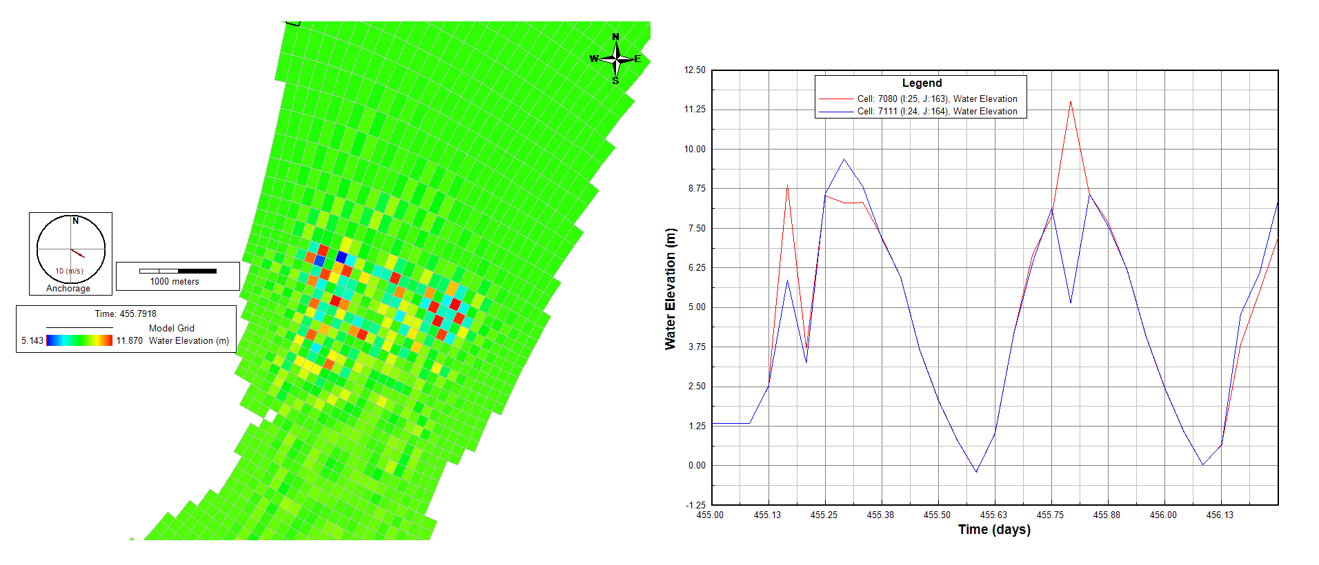
Water surface elevation plots: Look for evidence of spurious oscillations in the water surface elevation. This will often appear as a checkerboard pattern, where several adjacent cells may oscillate between high and low water surface elevations in a physically unrealistic manner.

Velocity magnitude/direction: Inspecting the predicted velocity magnitudes and directions can often be a useful way to evaluate model stability. Are the modeled velocity magnitudes realistic based on knowledge of the system? When a model is unstable or boundary conditions are not well configured, often high-velocity jets can be predicted by the model, which are artifacts of model instability. These jets may or may not result in the model crashing (often they cause a negative depth condition, which is a fatal error). So just because the model runs, it doesn’t mean that is always stable or producing reproducible results. Sometimes model grid cells adjacent to one another can exhibit considerable velocity magnitude and direction variations, which is another clear sign of instability in the model.
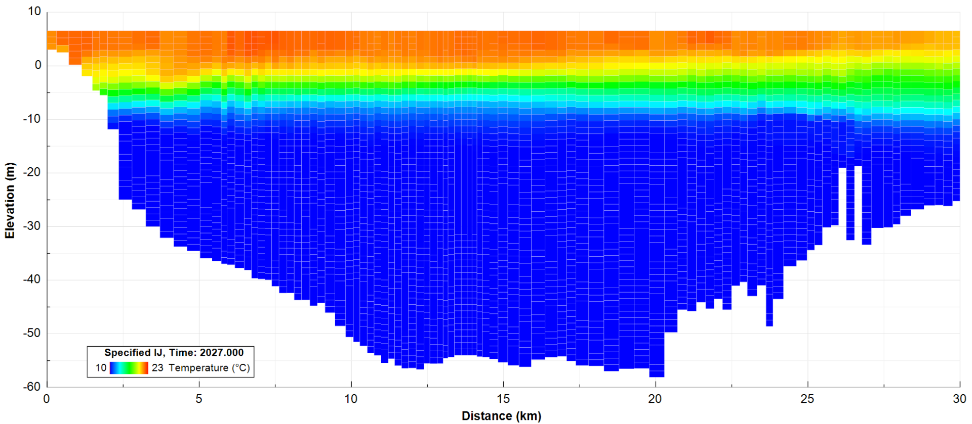
Density profile: In models with density, small instabilities in the internal model calculations can sometimes result in spurious oscillations in the density profile, resulting in overprediction of vertical mixing due to numerical diffusion. These spurious oscillations are sometimes associated with instabilities in water surface elevations but can occur independently even when velocity or water surface elevation predictions appear normal. For that reason, it is important to inspect vertical profiles and contour plots of the vertical structure along your model domain as shown in the 2DV image below (e.g. Figure 2).

Take an iterative approach
It is necessary to take an iterative approach to improve efficiency while maintaining stability. Often, the CFL timestep may be small relative to the maximum possible timestep, which allows for model stability/ convergence and reproducibility. However, determining the maximum timestep for your model is an iterative process. Usually, modest changes in the configuration of the dynamic time step can help you determine critical points at which the model may become unstable. You may then adjust those settings to ensure that the model behaves appropriately and that such a condition is less likely, or cannot occur.
For a fixed time step, sometimes you may find specific periods problematic due to highly dynamic changes (i.e., a large storm, hurricane, or significant discharge event). This instability may require smaller time steps to produce reasonable and realistic model predictions. In such a case, the model simulation may need to be segmented so that one period can be simulated with one fixed time step, and a second period can be configured with another time step. Such a process usually involves setting up model restart options and configuring the models such that a continuous period may be simulated using an initial cold start, followed by hot- or warm-start models thereafter.
Look out for our upcoming blogs that will discuss identifying bottlenecks in model simulations.


