Modeling Ice Formation in EEMS:
Part 1 – Introduction to the Heat-Coupled Ice Model and Demonstration Case
Introduction
Accurately simulating seasonal ice cover is crucial for understanding the hydrodynamics, primary production, and water quality of lake systems. The presence of ice cover, which inhibits wind stress, significantly influences the mixing and biogeochemical processes within lakes during winter. Moreover, the timing and extent of ice cover can affect the seasonal development of plankton communities, oxygen levels, and the occurrence of anoxia in the hypolimnion.
In this blog, we introduce an ice formation model based on the W2 framework (Wells and Cole, 2000). The model has been implemented in the three-dimensional EFDC+ code to simulate winter hydrodynamics and the thermal structure beneath the ice in aquatic systems. We also demonstrate the capability of this model through the simulation of ice formation in Lake Mendota, a freshwater eutrophic lake located in Madison, Wisconsin, USA.
Ice Module: Background Theory
Following the approach of Wells and Cole (2000), ice formation and melting in EFDC+ are simulated using the coupled heat-transfer model in the ice module. The heat-transfer option considers heat exchange between the ice cover and air, thermal conduction through the ice, heat conduction with the underlying water, and a “melt temperature” layer at the ice-water interface (Ashton, 1979). The overall heat balance for the water-ice system is given by the following equation:
\rho_i L_f \frac{\Delta h}{\Delta t} = h_{ai} \left( T_i – T_e \right) – h_{wi} \left( T_w – T_m \right)
where:
\rho_i = \text{density of ice (kg/m}^3\text{)}
L_f = \text{Latent heat of fusion of ice (J/kg)}
\frac{\Delta h}{\Delta t} = \text{Change in ice thickness } h \, (\text{m}) \text{ with time } t \, (\text{s})
h_{ai} = \text{coefficient of ice-to-air heat exchange (W/m}^2/^\circ\text{C)}
h_{wi} = \text{coefficient of water-to-ice heat exchange through melting (W/m}^2/^\circ\text{C)}
T_i = \text{ice temperature (°C)}
T_e = \text{equilibrium temperature of ice-to-air heat exchange (°C)}
T_w = \text{water temperature below ice (°C)}
T_m = \text{melt temperature (°C)}
Ice formation begins when surface water temperature is reduced to the freezing point through normal surface heat exchange processes. As heat continues to be removed, ice starts to form at the water’s surface. Any temperature drop below freezing is then converted into an equivalent ice thickness.
h_0 = \frac{-T_w L \rho_w C_w \Delta Z}{\rho_i L_f}
where:
h_0 = \text{thickness of initial ice formation (m)}
T_{wL} = \text{local temporary negative water temperature (°C)}
\Delta z = \text{layer thickness (m)}
\rho_w = \text{density of water (kg/m}^3\text{)}
C_{\rho w} = \text{specific heat of water (J/kg/°C)}
Ice growth and melting can occur at both the air-ice and ice-water interfaces. Heat fluxes at these interfaces are calculated based on the ice surface temperature, T_s, and the freezing temperature, T_f, which is set to 0°C for fresh water. Water is conserved in forming and melting ice. As ice forms, water is removed at a rate of 0.917 m³ for every 1 m³ of ice formed. This process reverses as the ice melts and returns water to the system.
Model Demonstration – Lake Mendota Case Study
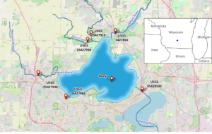
Lake Mendota is a freshwater eutrophic lake in southern Wisconsin, USA (Figure 1). It has a surface area of 39.61 km2 and a shoreline of 33.8 km. The lake has a mean depth of 12.8 m and a maximum depth of 25 m. Air temperature ranges between -39°C and 40°C, with an average of 8°C. Summer stratification commences in late April and lasts until October. In the winter months, thermal stratification takes place under the ice-covered surface. Lake Mendota’s volumetric properties are mainly driven by five inflow tributaries (Yahara River, Pheasant Branch, Sixmile Creek, Dorn Creek, and Spring Harbor) and one outlet stream (Yahara River).
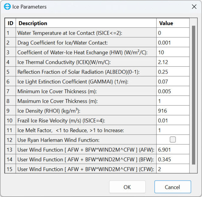
The model’s computational grid consists of 1,405 active water cells derived from a grid of 49 x 58 horizontal cells, with each cell measuring 170 x 170 m. A Sigma-Zed layering approach was applied, with the number of vertical layers varying between 3 and 30. The model was run for a 6-year period, from March 15, 2014, to June 15, 2020. The simulation employed a Heat-Coupled Ice model option, with the default ice parameter values is shown in Table 1.
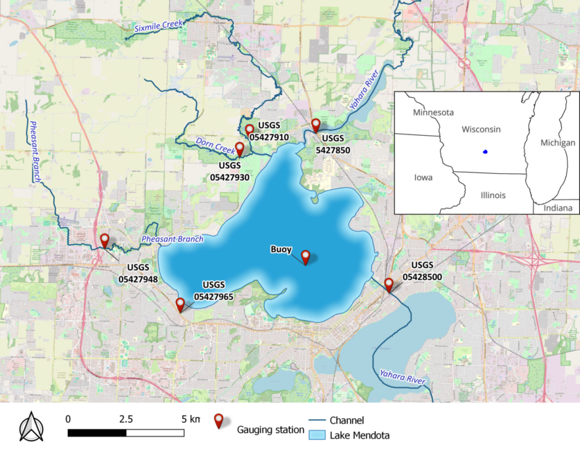
Table 1. Parameters used in the Heat Coupled Ice Model.
Ice Formation Results and Discussions
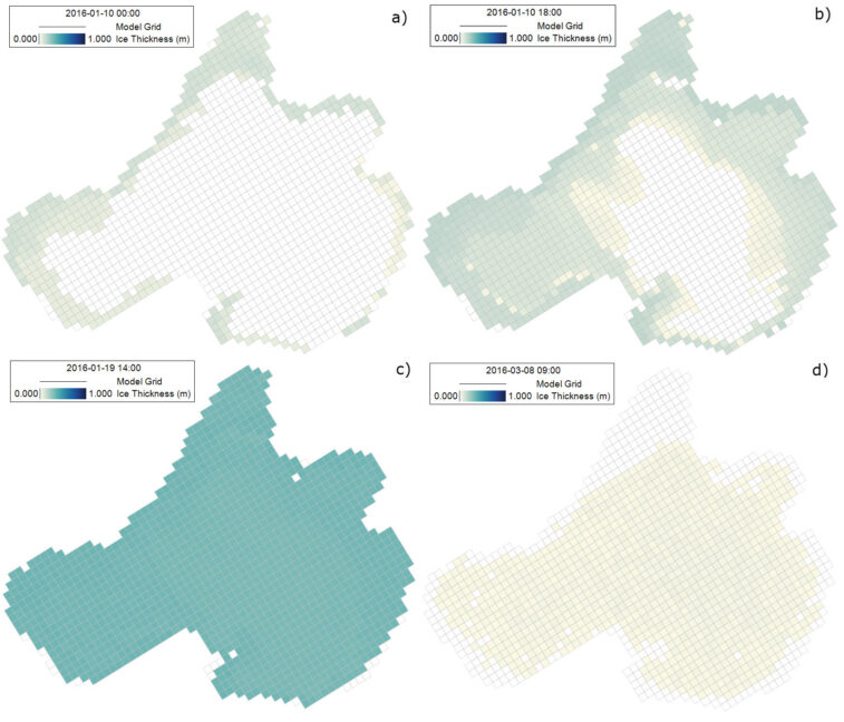
The cycle of ice formation and melting in Lake Mendota during the winter of 2015-2016 is illustrated by a series of snapshots shown in Figure 2. The numerical results indicate that ice begins forming along the shoreline. With sustained cold temperatures, the shoreline ice thickens and expands horizontally toward the middle of the lake. This spatial pattern aligns well with observations, as the shoreline is shallower, more exposed to cold air and wind, and therefore cools more quickly than the open water. Persistent ice coverage is also observed in the shallow areas along the northwest shore.
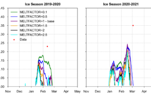
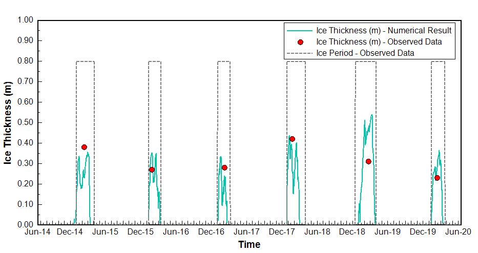
The simulated ice thickness is compared with observed data at Buoy Point from the winters of 2014 to 2020 in Figure 3. The maximum ice thickness ranged from 0.35 m to 0.55 m, depending on winter weather conditions. However, an overestimation of ice thickness was observed during the winter of 2018. Overall, the simulated ice thickness shows qualitative agreement with the observations. The model also successfully captured the duration of ice cover in most winter seasons. For this comparison, the ice formation period at Buoy Point was evaluated against observed data using a practical criterion: whether it was possible to row a boat between Picnic Point and Maple Bluff.
Conclusion
This blog introduces the coupled heat ice model implemented in the EFDC+ code. The model was validated using observed data from Lake Mendota in southern Wisconsin, USA. The results demonstrate the potential of using the EFDC+ ice formation capabilities to provide deeper insights into winter lake processes, such as thermal bars and inverse winter stratification. These processes significantly influence biogeochemistry but are challenging to observe when the water surface is covered by ice.

